5 分鐘看懂如何用卷積神經網路 CNN 判讀肺炎 CXR 影像

無論在醫院見實習當住院醫師，還是去診所做健檢業務或一般看診，胸腔 X 光影像（CXR）就跟每天都會刷牙洗臉吃飯如影隨形（咦 🤔？），尤其從 2019 年至今已經舉世造成極大影響的 COVID 就是從肺炎起家，各科英雄好漢懷疑病人有肺部感染時，除了兔寶寶戳鼻子採檢和血單、Culture 之外，就來張 CXR 起手式吧！

川流不息的病人、處理不完的 Complaints、堆積待打的病歷，此時電話那頭護理師提醒：「醫師可以幫我看一下 X 光片嗎？」

當然好 🖖！不過，如果有個小幫手可以先協助我做點功課，把五花八門的可能性縮減到較窄的範圍，好讓我點開 PACS 時已經有了初步的答案，是不是聽起來不錯呢？那麼，這次就讓我們來瞧瞧如何用 CNN 來建構肺炎閱片小幫手吧 👀

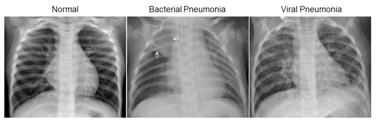
我們使用的是 Kaggle 肺炎胸腔 X 光資料集，來自於 2018 年發表在 Cell 學術期刊的論文，主要使用的是已經 Label 好的兒童胸部 X 光片，5,232 張影像裡分成 1,349 張正常、2,538 張細菌性肺炎、1,345 張病毒性肺炎的影像，大家可以點進去、下載資料集來玩玩看。

多元分類資料集的準備

如果大家已經下載了資料集，開始訓練模型前，我們先來看看手邊有哪些資料可以用。它已經很貼心地分好 Train / Validation / Test 三個資料夾，而每個資料夾裡又有「Normal」、「Pneumonia（肺炎）」兩種影像，Pneumonia 裡又根據檔名的註記，分為 Bacteria（細菌）與 Virus（病毒）兩個類別。

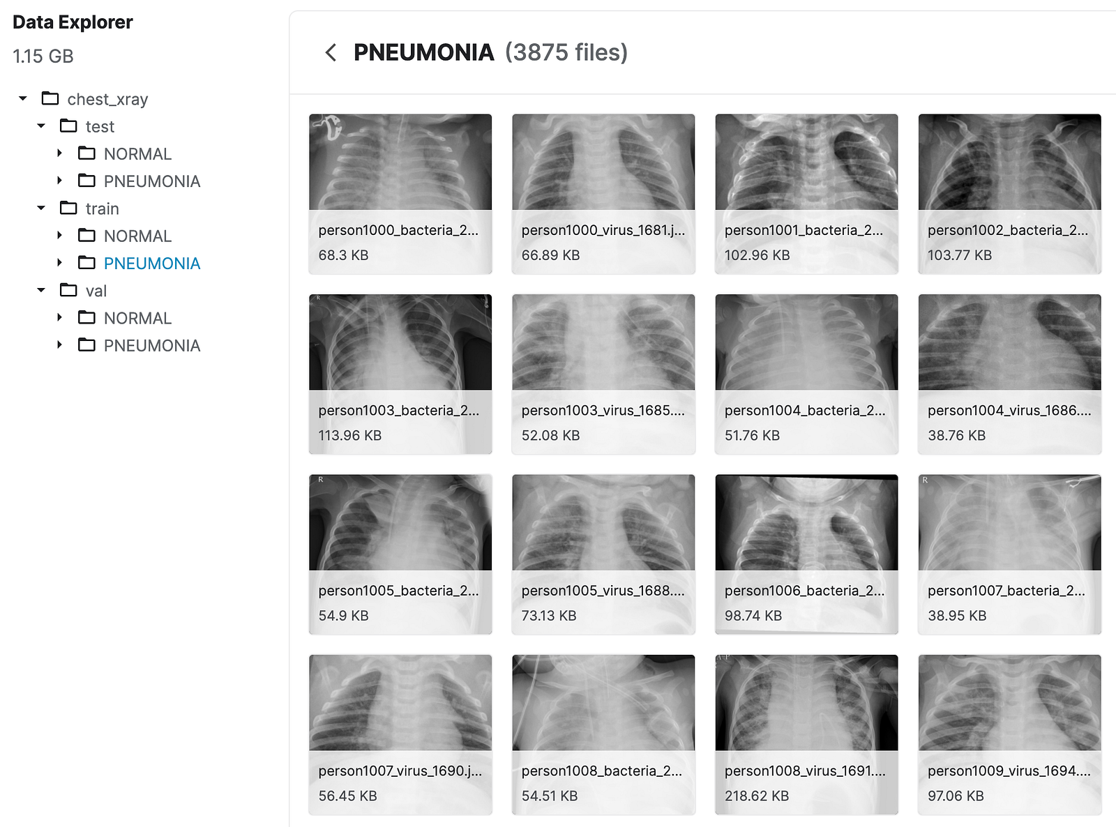
看完了資料長相，怎麼準備資料集呢？我們先來設定基本參數，如圖片大小固定成每張都是 200×200 再送給 Model、定義好 3 個類別（正常、細菌性、病毒性，當然也可以只分成正常和肺炎的二元分類），接著把圖片讀進來、以 for Loop 用路徑 Split 的方式指定每張圖片對應的分類。

IMG_SIZE = 200
all_class = ['normal', 'bacteria', 'virus']
class_map = {cls:i for i,cls in enumerate(all_class)} #  'normal':0, 'bacteria': 1, 'virus':2

# read all paths
img_paths_train = glob('chest_xray/train/*/*.jpeg')
img_paths_val = glob('chest_xray/val/*/*.jpeg')
img_paths_test = glob('chest_xray/test/*/*.jpeg')

# Resize img
img_resized = cv2.resize(img, (IMG_SIZE, IMG_SIZE))

def read_data(paths):
    data_count = len(paths)
    x = np.zeros((data_count, IMG_SIZE, IMG_SIZE, 3))
    y = np.zeros((data_count, ))

    for i, path in tqdm(enumerate(paths)):
        # read image
        img = cv2.imread(path)
        img = cv2.resize(img, (IMG_SIZE, IMG_SIZE)) # resize
        img = img / 255. # normalization

        # read class index
        cls = path.split(os.sep)[-2]
        # for pneumonia class
        if cls == 'pneumonia':
            # get filename
            filename = path.split(os.sep)[-1]
            # get pneumonia class
            cls_pneumonia = filename.split('_')[1] 
            cls_idx = class_map[cls_pneumonia]
        # for normal class
        else:
            cls_idx = class_map[cls]
        x[i] = img
        y[i] = cls_idx
    return x, y
    
x_train, y_train = read_data(img_paths_train)
x_val, y_val = read_data(img_paths_val)

不過我們現在 y 裡裝的只有最開始 class_map 的 0, 1, 2，要做 one-hot encoding 轉為長度 = 3（分幾類決定了長度）的向量，用 keras 的 utils 中to_categorical 這個 Function。

# one-hot encoding
y_train = utils.to_categorical(y_train, num_classes=len(class_map))
y_val = utils.to_categorical(y_val, num_classes=len(class_map))
y_test = utils.to_categorical(y_test, num_classes=len(class_map))

建構模型

準備好資料以後，就來建模吧！要特別注意，餵給模型的 Data Input Size，形狀必須跟我們原本資料集 x_train, x_val, x_test 一樣才行。以下面這個模型為例，前兩層的卷積我們使用 64 個 Filters、Kernel Size 是 3×3、Activation Function 用 Relu，接著加上 1 層 MaxPooling…重複再用 2 層分別有 128、256、512 個 Filters 的卷積加上 1 層 MaxPooling，最後把 Feature Maps 的特徵向量攤平 Flatten、接上 1 層 Dense Layer，分成 3 類、以 softmax 輸出模型結果。

inputs = layers.Input(shape=(IMG_SIZE, IMG_SIZE, 3))
x = layers.Conv2D(filters=64, kernel_size=3, activation='relu')(inputs)
x = layers.Conv2D(filters=64, kernel_size=3, activation='relu')(x)
x = layers.MaxPool2D(2)(x)
x = layers.Conv2D(filters=128, kernel_size=3, activation='relu')(x)
x = layers.Conv2D(filters=128, kernel_size=3, activation='relu')(x)
x = layers.MaxPool2D(2)(x)
x = layers.Conv2D(filters=256, kernel_size=3, activation='relu')(x)
x = layers.Conv2D(filters=256, kernel_size=3, activation='relu')(x)
x = layers.MaxPool2D(2)(x)
x = layers.Conv2D(filters=512, kernel_size=3, activation='relu')(x)
x = layers.Conv2D(filters=512, kernel_size=3, activation='relu')(x)
x = layers.MaxPool2D(2)(x)
x = layers.Flatten()(x)
x = layers.Dense(64, activation='relu')(x)
prediction = layers.Dense(3, activation='softmax')(x)
model = models.Model(inputs=inputs, outputs=prediction)

訓練模型

建模後，我們設定讓模型計算 Loss、優化超參數、衡量結果的指標，用分類的損失函數 categorical_crossentropy、Optimizer 用預設的 SGD（Stochastic Gradient Descent）、計算模型的 Accuracy，再設定 Batch Size、Epochs 的數量。

model.compile(loss=tf.keras.losses.categorical_crossentropy,
              optimizer=tf.keras.optimizers.SGD(),
              metrics=['accuracy'])
              
logs = model.fit(x_train, y_train,
                batch_size=32,
                epochs=50,
                verbose=1,
                validation_data=(x_val, y_val),
                 )

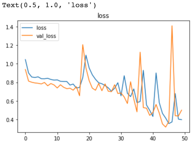
跑完之後，我們找出訓練歷程中 Validation Loss 最低是多少、對應的 Accuracy 有多高，再把 Training（藍色線）、Validation 隨著 50 個 Epochs 的 Iterations，Accuracy 和 Loss 的變化是多少；通常 Training 的 Loss 會比較低。

min_loss_epoch = np.argmin(history['val_loss'])
print('val loss ', history['val_loss'][min_loss_epoch])
print('val acc', history['val_accuracy'][min_loss_epoch])

plt.plot(history['accuracy'])
plt.plot(history['val_accuracy'])
plt.legend(['accuracy', 'val_accuracy'])
plt.title('accuracy')

plt.plot(history['loss'])
plt.plot(history['val_loss'])
plt.legend(['loss', 'val_loss'])
plt.title('loss')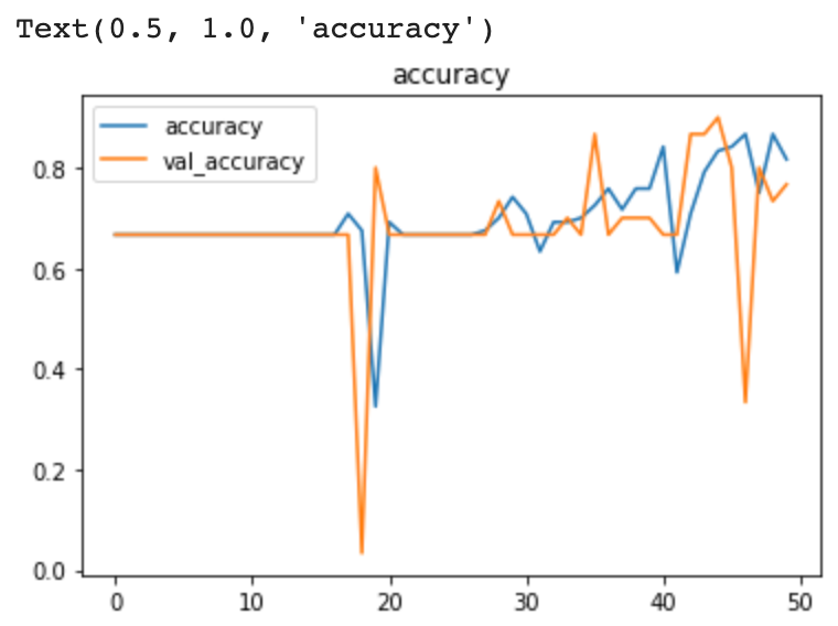

衡量模型的其他 Metrics

sklearn 有提供分類任務裡常用的 classification_report、Confusion Matrix，我們用模型沒看過的資料（x_test），讓模型預測每一筆資料的機率值，再透過 argmax 看哪一個類別有最大的機率（y_pred），去跟 Ground Truth（y_true）來評估成果如何。像我們總體的 Accuracy 只有 0.6，第 0 類表現最好（0.73）、第 1 類表現最糟（0.41）。

from sklearn.metrics import classification_report, confusion_matrix

y_true = np.argmax(y_test, axis=-1)
prediction = model.predict(x_test)
y_pred = np.argmax(prediction, axis=-1)

# classification_report
print(classification_report(y_true, y_pred))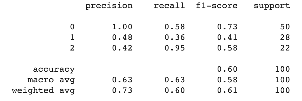

希望這次的分享大家覺得有意思，下次再讓我們繼續看看 AI 遇上臨床工作人員，有什麼令人怦然心動的火花吧 🌹

#CC